20 Example 7.3 OGATA 4edition (step input, ramp input, lag-lead compensator)

Laplace.T	Root-locus	Transient response	Frecuency response

20 Example 7.3 OGATA 4edition (step input, ramp input, lag-lead compensator)

Let's solve the problem of the book otherwise. The open-loop transfer function is:

$\begin{displaymath}G(s)=\frac{4}{s\cdot (s+0.5)}\end{displaymath}$

We calculate the dominant pole
The damped ratio is 0.5 and the damped natural frecuency is 5. Therefore, the dominant pole must be:

$\begin{displaymath}s_{1}=-0.5\cdot 5+j5\cdot \sqrt{1-0.5^{2}}=-2.5\pm j4.33\end{displaymath}$

We calculate the angle to correct:

$\begin{displaymath}G(s1)= - 0.0967033 + 0.1370414j \end{displaymath}$

$\begin{displaymath}\lfloor{G(s_{1})}=(180-arctg\left(\frac{0.137}{0.0967} \right))=125.20872 \end{displaymath}$

$\begin{displaymath}\phi=180-125.20872=54.791281 \end{displaymath}$

Calculate $T_{1}$ y $\gamma$

$\begin{displaymath}\lfloor{ \frac{s_{1}+\frac{1}{T_{1}}}{s_{1}+\frac{\gamma}{T_{1}}} }=54.791281 \end{displaymath}$

We will place the zero in -2.5 . Aligned with the dominant pole.

$\begin{displaymath}d\cdot cos(54.79)=4.33\end{displaymath}$

$\begin{displaymath}l=d\cdot sen(54.79)=4.33 \cdot tg(54.79)=6.1363636 \end{displaymath}$

$\begin{displaymath}p1=-2.5-l=-8.6363636\end{displaymath}$

Zero: -2.5 and pole: -8.63.
Therefore the lead-compensator is

$\begin{displaymath}K_{c}\cdot \frac{s+\frac{1}{T_{1}}}{s+\frac{\gamma}{T_{1}}}=K_{c}\cdot \frac{s+2.5}{s+8.63} \end{displaymath}$

We can calculate the value of $\gamma$

$\begin{displaymath}\frac{1}{T_{1}}=2.5;\frac{\gamma}{T_{1}}=8.63\end{displaymath}$

$\begin{displaymath}\gamma \cdot 2.5=8.63;\gamma=\frac{8.63}{2.5}=3.45\end{displaymath}$

Let us calculate the value of $K_{c}$

$\begin{displaymath}\left\vert K_{c}\cdot \frac{s_{1}+2.5}{s_{1}+8.63} \cdot \frac{4}{s_{1}\cdot (s_{1}+0.5)}\right\vert=1\end{displaymath}$

$\begin{displaymath}K_{c}=\frac{1}{0.097}=10.34\end{displaymath}$

The obtained lead-compensator is:

$\begin{displaymath}10.34\cdot \frac{s+2.5}{s+8.63}\end{displaymath}$

Let us calculate the $\beta$ of lag compensator. Knowing

$\begin{displaymath}\frac{s+\frac{1}{T_{2}}}{s+\frac{1}{\beta\cdot T_{2}}}\end{displaymath}$

$\begin{displaymath}\lim_{s\rightarrow 0}(s\cdot \frac{4}{s\cdot (s+0.5)} \cdot \frac{\beta}{\gamma}\cdot K_{c})=23.95\cdot \beta=K_{v}=80\end{displaymath}$

$\begin{displaymath}\beta=\frac{80}{23.95}=3.34\end{displaymath}$

Choosing $T_{2}=5$ as in the book, we will see that compensator's conditions are ok

$\begin{displaymath}\frac{s+\frac{1}{5}}{s+\frac{1}{3.34\cdot 5}}=\frac{s+0.2}{s+0.06}\end{displaymath}$

$\begin{displaymath}\left\vert\frac{s_{1}+0.2}{s_{1}+0.06} \right\vert=0.986\approx 1\end{displaymath}$

$\begin{displaymath}\lfloor\left( \frac{s_{1}+0.2}{s_{1}+0.06}\right)=-1.42º\end{displaymath}$

$\begin{displaymath}-5º<-1.42<0º\end{displaymath}$

The conditions are ok. The obtained lag-lead compensator is

$\begin{displaymath}10.34\cdot \frac{s+2.5}{s+8.63}\cdot \frac{s+0.2}{s+0.06}\end{displaymath}$

Let us draw the response of the system to unit-step input. Also showing the code of all the load obtained.
Program in Scilab:
s=%s;
g=4/(s*(s+0.5));
s1=-2.5+5*sqrt(1-0.5^2)*%i;
gs=syslin('c',g);

//angle's system in dominant pole s1
gs1=horner(gs,s1);
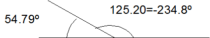
angulo=180-360*atan(abs(imag(gs1))/abs(real(gs1)))/(2*%pi)
angulocorregir=180-angulo

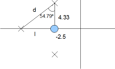
//lead-pole
l=imag(s1)*tan(2*%pi*angulocorregir/360);
p1=-2.5-l;
z1=-2.5;
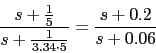
gc=(s-z1)/(s-p1)

//the gain of compensator
gma=p1/z1;
gt=gc*g;
aux1=(abs(horner(gt,s1)));
kc=1/aux1


//lag compensator
gct=kc*gc;
gt2=kc*gt;
aux3=s*gt2;
aux4=horner(aux3,0);
b=80/aux4
gc2=(s+(1/5))/(s+(1/(5*b)))

//Check results
aux5=horner(gc2,s1);
aux6=abs(aux5)
angulo2=-360*atan(abs(imag(aux5))/abs(real(aux5)))/(2*%pi)

//Draw responses
gt3=gc2*gt2;
gct2=6.26*((s+0.5)/(s+5.02))*((s+0.2)/(s+0.01247));
gt4=g*gct2;
gct3=10*((s+2.38)/(s+8.34))*((s+0.1)/(s+0.0285));
gt5=g*gct3;
t=0:0.01:5;
glc=g /. 1;
glc1=gt3 /. 1;
glc2=gt4 /. 1;
glc3=gt5 /. 1;
y=csim('step',t,glc);
y1=csim('step',t,glc1);
y2=csim('step',t,glc2);
y3=csim('step',t,glc3);
clf;

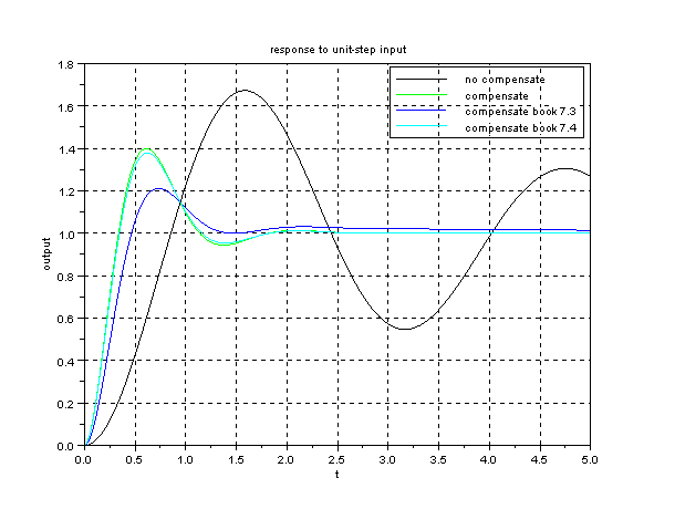
plot(t,y,'k');

plot(t,y1,'g');

plot(t,y2,'b');

plot(t,y3,'c');
legend(['no compensate';'compensate';'compensate book 7.3'
;'compensate book 7.4']);

xtitle('response to unit-step input',
't','output');
xgrid;
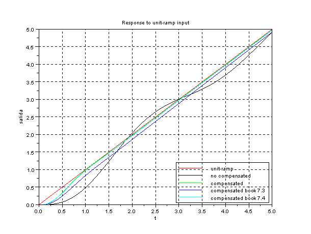
Let us draw the response to unit-ramp.

let us add more code lines:
y=csim(t,t,glc);
y1=csim(t,t,glc1);
y2=csim(t,t,glc2);
y3=csim(t,t,glc3);
clf;
plot(t,t,'r');

plot(t,y,'k');

plot(t,y1,'g');

plot(t,y2,'b');

plot(t,y3,'c');
legend(['unit-ramp';'no compensated';'compensated'
;'compensated book 7.3';'compensated book 7.4'],style=4);

xtitle('Response to unit-ramp input'
,'t','salida');

xgrid;