21 Problem A9.9 OGATA 4ed(Lag-lead Compensator)

Laplace.T	Root-locus	Transient response	Frecuency response

21 Problem A9.9 OGATA 4ed(Lag-lead Compensator)
Let us calculate a lag-lead compensator that satisfies the following requirements static velocity constant error $K_{v}=10$ , phase margin 50 and gain margin $\geq 10dB$ . The open-loop system is the following:

$\begin{displaymath}G(s)=\frac{1}{s\cdot (s+1)\cdot (s+4)}\end{displaymath}$
First, let's calculate the value of K to obtain $G_{1}(s)$

$\begin{displaymath}K_{v}=\lim_{s \rightarrow 0}{s\cdot K_{c}\cdot G(s)}=\frac{K_{c}}{4}=\frac{K}{4}=10\end{displaymath}$

$\begin{displaymath}K=40\end{displaymath}$

$\begin{displaymath}G_{1}(s)=\frac{40}{s\cdot (s+1)\cdot (s+4)}=\frac{10}{s\cdot (s+1) \cdot (\frac{s}{4}+1) }\end{displaymath}$
Let's calculate Bode plot $G_{1}(jw)$
Gain table:

$\begin{displaymath}20\cdot log(10)=20\end{displaymath}$

w 1 4

$\frac{1}{s}$ (-20) 0 (-20) (-20)

$\frac{1}{ (s+1)}$ (0) 0 (-20) (-20)

$\frac{1}{(\frac{s}{4}+1)}$ (0) 0 (0) 0 (-20)

(-20) 20 (-40) -4.06 (-60)

$\begin{displaymath}dB\vert G_{1}(j0.1)\vert=20-20\cdot log(0.1)=40\end{displaymath}$

$\begin{displaymath}dB\vert G_{1}(j4)\vert=20-40\cdot log (\frac{4}{1})=-4.06\end{displaymath}$

Phase table:

w 0.1 0.4 1 4 10 40

$\frac{1}{s}$ -90 (0) -90 (0) -90 (0) -90 (0) -90 (0) -90 (0)

$\frac{1}{ (s+1)}$ 0 (-45) (-45) -45 (-45) (-45) -90 (0) -90 (0)

$\frac{1}{(\frac{s}{4}+1)}$ 0 (0) 0 (-45) (-45) -45 (-45) (-45) -90 (0)

-90 (-45) -117 (-90) -153 (-90) -207 (-90) -243 (-45) -270 (0)

$\begin{displaymath}\lfloor{G_{1}(j0.1)}=-90\end{displaymath}$

$\begin{displaymath}\lfloor{G_{1}(j0.4)}=\lfloor{G_{1}(j0.1)}-45 \cdot log(\frac{0.4}{0.1})=-117\end{displaymath}$

$\begin{displaymath}\lfloor{G_{1}(j1)}=\lfloor{G_{1}(j0.4)}-90 \cdot log(\frac{1}{0.4})=-152.9\end{displaymath}$

$\begin{displaymath}\lfloor{G_{1}(j4)}=\lfloor{G_{1}(j0.4)}-90 \cdot log(\frac{4}{0.4})=-207\end{displaymath}$

$\begin{displaymath}\lfloor{G_{1}(j10)}=\lfloor{G_{1}(j0.4)}-90 \cdot log(\frac{10}{0.4})=-242.9\end{displaymath}$

$\begin{displaymath}\lfloor{G_{1}(j40)}=-270\end{displaymath}$

$\begin{displaymath}\lfloor{G_{1}(j100)}=-270\end{displaymath}$

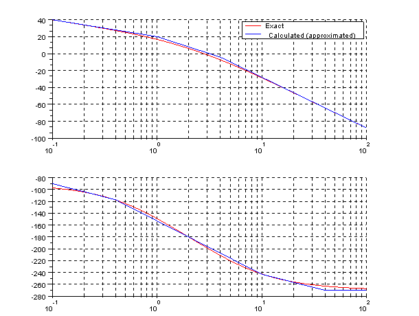
Calculations and Bode plot by Scilab
w1=[0.1 1 4 40 100];
w2=[0.1 0.4 1 4 10 40 100];

gdb1=20*log10(10)
gdb(1)=gdb1-20*log10(0.1)
gdb(2)=gdb1
gdb(3)=gdb1-40*log10(4)
gdb(4)=gdb(3)-60*log10(40/4)
gdb(5)=gdb(3)-60*log10(100/4)

a(1)=-90
a(2)=a(1)-45*log10(0.4/0.1)
a(3)=a(2)-90*log10(1/0.4)
a(4)=a(2)-90*log10(4/0.4)
a(5)=a(2)-90*log10(10/0.4)
a(6)=a(5)-45*log10(40/10)
a(7)=a(6)

s=%s/(%pi*2);
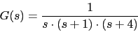
g=40/(s*(s+1)*(s+4));
gs=syslin('c',g);
w=logspace(-1,2,100);
gsf=tf2ss(gs);
[frq1,rep] =repfreq(gsf,w);
[db,phi]=dbphi(rep);

clf;
subplot(2,1,1);
plot2d(w,db,5,logflag="ln")
plot2d(w1,gdb,2,logflag="ln")
legends(['Exact','Calculated (approximated)'],[5,2],opt=1);
xgrid;
subplot(2,1,2);
plot2d(w,phi,5,logflag="ln")
plot2d(w2,a,2,logflag="ln")
xgrid;
Let's calculate the frequency to which $G_{1}(jw )$ phase is -180. This is the new gain crossover frequency.

$\begin{displaymath}-180=\lfloor{G_{1}(j0.4)}-90 \cdot log(\frac{nwcg}{0.4})\end{displaymath}$

$\begin{displaymath}-180=-117-90 \cdot log(\frac{nwcg}{0.4})\end{displaymath}$

$\begin{displaymath}nwcg=2\end{displaymath}$

The value $\frac{1}{T_{2}}$ of lag compensator is a decade below the new gain crossover frequency

$\begin{displaymath}\frac{1}{T_{2}}=\frac{2}{10}=0.2\end{displaymath}$
The phase margin is , with this value we calculate $\beta$

$\begin{displaymath}\alpha=\frac{1}{\beta}\end{displaymath}$

$\begin{displaymath}sen(55)=\frac{1-\alpha}{1+\alpha}\end{displaymath}$

$\begin{displaymath}\alpha=\frac{1-sen(55)}{1+sen(55)}=0.099\end{displaymath}$

$\begin{displaymath}\beta=10.06\end{displaymath}$

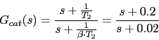
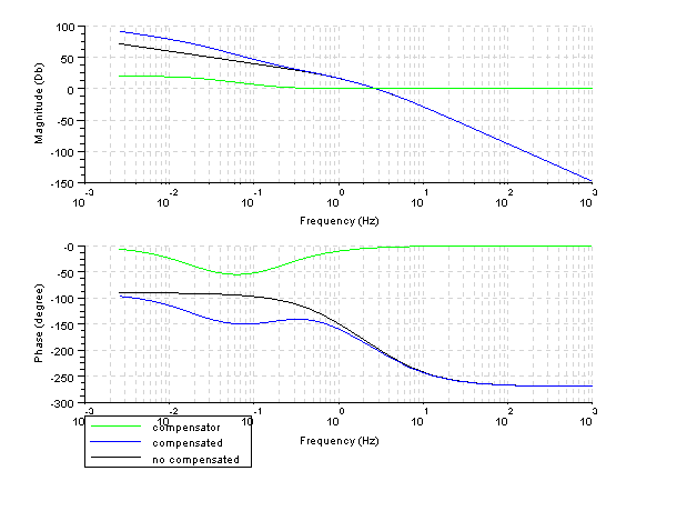
The lag compensator is:

$\begin{displaymath}G_{cat}(s)=\frac{s+\frac{1}{T_{2}}}{s+\frac{1}{\beta\cdot T_{2}}}=\frac{s+0.2}{s+0.02}\end{displaymath}$

We draw the lag compensator by Scilab

Scilab program:
s=%s/(2*%pi);
g=40/(s*(s+1)*(s+4));
gc1=(s+0.2)/(s+0.02);
gt1=g*gc1;
gs=syslin('c',g);
gc1s=syslin('c',gc1);
gt1s=syslin('c',gt1);
clf();
bode([gs;gt1s;gc1s],['compensator';'compensated';'no compensated']);
Let's calculate the lead compensator. We calculate the $G_{1}(jw)$ gain in new gain crossover frequency.

$\begin{displaymath}dB\vert G_{1}(j2)\vert=dB\vert G_{1}(1)\vert-40\cdot log (\frac{2}{1})=7.95\end{displaymath}$

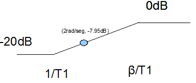
We calculate the pole and zero of compensator, draw a line passing a line through point (2rad/seg,-7.95dB) of Bode plot and see where intersects with line -20dB(gain value of lag compensator in $\frac{1}{\beta \cdot T}$ ) and line 0dB. The slope is 20dB/dec.

$\begin{displaymath}-7.95+20\cdot log(\frac{w_{2}}{2})=0\end{displaymath}$

$\begin{displaymath}\frac{w_{2}}{2}=10^{\frac{7.95}{20}}\end{displaymath}$

$\begin{displaymath}w_{2}=2\cdot 10^{\frac{7.95}{20}}=5rad/seg=\frac{\beta}{T_{1}}\end{displaymath}$

$\begin{displaymath}-20+20\cdot log(\frac{2}{w_{1}})=-7.95\end{displaymath}$

$\begin{displaymath}\frac{2}{w_{1}}=10^{\frac{12.05}{20}}\end{displaymath}$

$\begin{displaymath}w_{1}=\frac{2}{10^{\frac{12.05}{20}}}=0.5rad/seg=\frac{1}{T_{1}}\end{displaymath}$

The lead compensator is:

$\begin{displaymath}G_{cad}(s)=40\cdot \frac{s+0.5}{s+5}\end{displaymath}$

Let's calculate the phase and gain margins, and Bode plot by Scilab

Scilab program:
s=%s/(2*%pi);
g=40/((s+0.00000000001)*(s+1)*(s+4));
gc1=(s+0.2)/(s+0.02);
gc2=(s+0.5)/(s+5);
gc3=(s+0.4)*(s+0.2)/((s+4)*(s+0.02));
gt1=g*gc1*gc2;
gt2=gc3*g;
gs=syslin('c',g);
gc1s=syslin('c',gc1*gc2);
gc2s=syslin('c',gc3);
gt1s=syslin('c',gt1);
[mg,fcp]=g_margin(gt1s)
[mp,fcg]=p_margin(gt1s)

gt2s=syslin('c',gt2);
clf();
bode([gs;gt1s;gc1s;gc2s;gt2s],['compensated (book)';'Compensator (book)';
'compensator';'compensated';'no compensated']);
Results:
-->[mg,fcp]=g_margin(gt1s)
 fcp  =
 
    4.7720943  
 mg  =
 
    14.341752  
 
-->[mp,fcg]=p_margin(gt1s)
 fcg  =
 
    1.5842083  
 mp  =
 
    59.086358
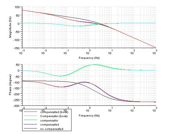
As we see the gain margin is 14dB >10dB and phase margin is 59>50

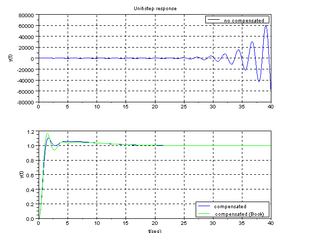
Lets draw the unit-step response by Scilab

Scilab program:
s=%s;
g=40/(s*(s+1)*(s+4));
gc1=(s+0.2)/(s+0.02);
gc2=(s+0.5)/(s+5);
gc3=(s+0.4)*(s+0.2)/((s+4)*(s+0.02));
gt1=g*gc1*gc2;
gt2=gc3*g;
glc=g /. 1;
glc2=gt1 /. 1;
glc3=gt2 /. 1;
gs=syslin('c',glc);
gs2=syslin('c',glc2);
gs3=syslin('c',glc3);
t=0:0.1:40;
y=csim('step',t,gs);
y2=csim('step',t,gs2);
y3=csim('step',t,gs3);
clf();
subplot(2,1,1);
plot(t,y,1);
legends('no compensated',1,opt=1)
xgrid;
xtitle('Unit-step response','','y(t)')
subplot(2,1,2)
plot(t,y2,'b');
plot(t,y3,'g');
legends(['compensated';'compensated (Book)'],[2;3],opt=4);
xtitle('','t(seg)','y(t)')
xgrid;
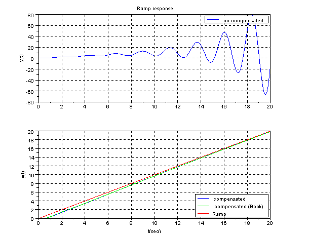
Let's draw the ramp response by Scilab.

Scilab program:
s=%s;
g=40/(s*(s+1)*(s+4));
gc1=(s+0.2)/(s+0.02);
gc2=(s+0.5)/(s+5);
gc3=(s+0.4)*(s+0.2)/((s+4)*(s+0.02));
gt1=g*gc1*gc2;
gt2=gc3*g;
glc=g /. 1;
glc2=gt1 /. 1;
glc3=gt2 /. 1;
gs=syslin('c',glc);
gs2=syslin('c',glc2);
gs3=syslin('c',glc3);
t=0:0.1:20;
y=csim(t,t,gs);
y2=csim(t,t,gs2);
y3=csim(t,t,gs3);
clf();
subplot(2,1,1);
plot(t,y,1);
legends('no compensated',2,opt=1)
xgrid;
xtitle('Ramp response','','y(t)')
subplot(2,1,2)
plot(t,t,'r');
plot(t,y2,'b');
plot(t,y3,'g');
legends(['compensated';'compensated (Book)';'Ramp'],[2;3;5],opt=4);
xtitle('','t(seg)','y(t)')
xgrid;