22 Problem A9.10 OGATA 4ed(PID compensator)

Laplace.T	Root-locus	Transient response	Frecuency response

22 Problem A9.10 OGATA 4ed(PID compensator)

$K_{v}=4$

$\geq 10dB$

$\begin{displaymath}G(s)=\frac{1}{(s^{2}+1)}\end{displaymath}$

Let's draw the bode plot by Scilab of:

$\begin{displaymath}G_{1}(s)=\frac{4}{(s^{2}+1)}\end{displaymath}$

Scilab program:

s=%s/(2*%pi);
g=4/(s*(s^2+1));
gs=syslin('c',g);
clf();
bode(gs,0.1,10);

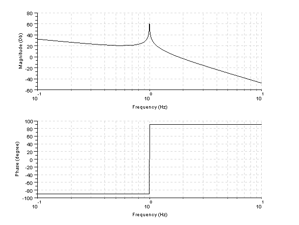
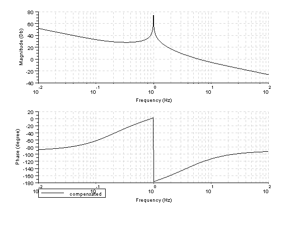
Let's draw the bode plot by Scilab of:

$\begin{displaymath}G_{1}(s)\cdot G_{ad}=\frac{4}{(s^{2}+1)}\cdot (5\cdot s+1)\end{displaymath}$

Scilab program:

s=%s/(2*%pi);
g=4/(s*(s^2+1));
gcad=(5*s+1);
gs=syslin('c',g);
gs2=syslin('c',g*gcad);
clf();
bode(gs2,'compensated');

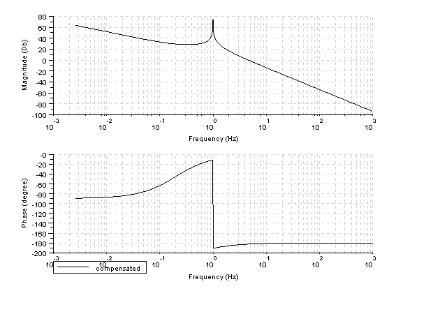
Let's draw the bode plot by Scilab of:

$\begin{displaymath}G_{1}(s)\cdot G_{ad}=\frac{4}{(s^{2}+1)}\cdot (5\cdot s+1)\cdot (0.25\cdot s+1)\end{displaymath}$

Scilab program:

s=%s/(2*%pi);
g=4/(s*(s^2+1));
gcad=(5*s+1);
gcad2=(0.25*s+1);
gs=syslin('c',g);
gs2=syslin('c',g*gcad*gcad2);
clf();
bode(gs2,0.01,100,'compensated');

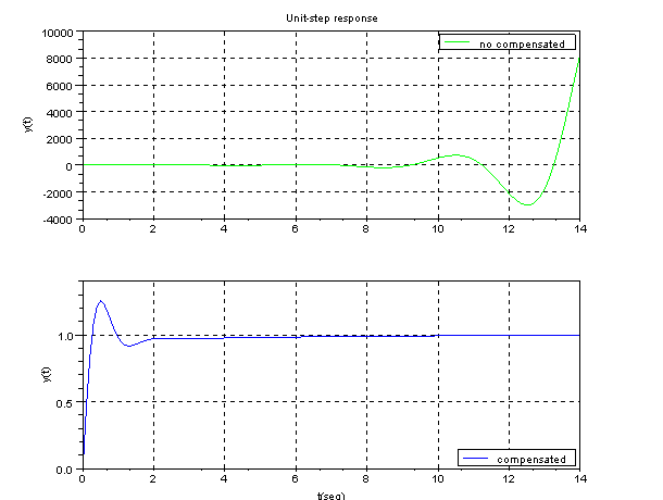
Let's draw the unit-step response by Scilab.

Scilab program:

s=%s;
g=4/(s*(s^2+1));
gcad=(5*s+1);
gcad2=(0.25*s+1);
gt1=g*gcad*gcad2;
glc=g /. 1;
glc2=gt1 /. 1;
gs=syslin('c',glc);
gs2=syslin('c',glc2);
t=0:0.1:14;
y=csim('step',t,gs);
y2=csim('step',t,gs2);
clf();
subplot(2,1,1);
plot(t,y,'g');
legends('no compensated',3,opt=1)
xgrid;
xtitle('Unit-step response','','y(t)')
subplot(2,1,2)
plot(t,y2,'b');
legends('compensated',2,opt=4);
xtitle('','t(seg)','y(t)')
xgrid;

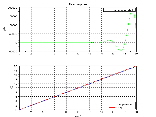
Let's draw the ramp response by Scilab.

Scilab program:

s=%s;
g=4/(s*(s^2+1));
gcad=(5*s+1);
gcad2=(0.25*s+1);
gt1=g*gcad*gcad2;
glc=g /. 1;
glc2=gt1 /. 1;
gs=syslin('c',glc);
gs2=syslin('c',glc2);
t=0:0.1:20;
y=csim(t,t,gs);
y2=csim(t,t,gs2);
clf();
subplot(2,1,1);
plot(t,y,'g');
legends('no compensated',3,opt=1)
xgrid;
xtitle('Ramp response','','y(t)')
subplot(2,1,2)
plot(t,y2,'b');
plot(t,t,'r');
legends(['compensated';'ramp'],[2;5],opt=4);
xtitle('','t(seg)','y(t)')
xgrid;