17 Problem A9.3 OGATA 4ed(Lead compensator, Bode plot)

Laplace.T	Root-locus	Transient response	Frecuency response

17 Problem A9.3 OGATA 4ed(Lead compensator, Bode plot)
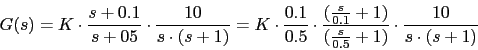
We want the phase margin equal to 60. Let's calculate K.

$\begin{displaymath}G(s)=K\cdot \frac{s+0.1}{s+0.5}\cdot \frac{10}{s\cdot (s+1)}\end{displaymath}$

Solution:

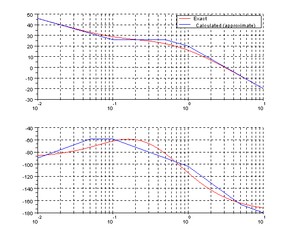
$\begin{displaymath}G(s)=K\cdot \frac{s+0.1}{s+05}\cdot \frac{10}{s\cdot (s+1)}=K... ...rac{s}{0.1}+1)}{(\frac{s}{0.5}+1)}\cdot \frac{10}{s\cdot (s+1)}\end{displaymath}$

Let's calculate the system's Bode plot.

Gain table:

$\begin{displaymath}20\cdot log(\frac{10\cdot 0.1}{0.5})=20\cdot log(2)=6.02\end{displaymath}$

w 0.1 0.5 1

$(\frac{s}{0.1}+1)$ (0) 0 (20) ( 20) (20)

$\frac{1}{ (\frac{s}{0.5}+1)}$ (0) 0 (0) 0 (-20) (-20)

$\frac{1}{ s}$ (-20) (-20) (-20) 0 (-20)

$\frac{1}{( s+1)}$ (0) 0 (0) 0 (0) 0 (-20)

$db \vert G(jw)\vert$ (-20) 26 (0) 26 (-20) 20 (-40)

$\begin{displaymath}dB\vert G_{1}(j0.01)\vert=6.02-20\cdot log(0.01)=46.02\end{displaymath}$

$\begin{displaymath}dB\vert G_{1}(j0.1)\vert=6.02-20\cdot log(0.1)=26.02\end{displaymath}$

$\begin{displaymath}dB\vert G_{1}(j1)\vert=26-20\cdot log (\frac{1}{0.5})=20\end{displaymath}$

$\begin{displaymath}dB\vert G_{1}(j10)\vert=20-40\cdot log (\frac{10}{1})=-20\end{displaymath}$

Phase table:

w 0.01 0.05 0.1 0.5 1 5 10

$(\frac{s}{0.1}+1)$ (0) 0 (45) (45) 45 (45) (45) 90 (0) 90 (0) 90

$\frac{1}{ (\frac{s}{0.5}+1)}$ (0) 0 (0) 0 (-45) (-45) -45 (-45) (-45) -90 (0) -90

$\frac{1}{ s}$ (0) -90 (0) -90 (0) -90 (0) -90 (0) -90 (0) -90 (0) -90

$\frac{1}{( s+1)}$ (0) 0 (0) 0 (0) 0 (-45) (-45) -45 (-45) (-45) -90

$\lfloor{G(jw)}$ (0) -90 (45) -58 (0) -58 (-45) -90 (-45) -103 (-90) -166 (-45) -180

$\begin{displaymath}\lfloor{G(j0.05)}=-90+45\cdot log(\frac{0.05}{0.01})=-58.55\end{displaymath}$

$\begin{displaymath}\lfloor{G(j0.1)}=-58.55\end{displaymath}$

$\begin{displaymath}\lfloor{G(j0.5)}=-58.55-45\cdot log(\frac{0.5}{0.1})=-90\end{displaymath}$

$\begin{displaymath}\lfloor{G(j1)}=-58.55-45\cdot log(\frac{1}{0.1})=- 103.55\end{displaymath}$

$\begin{displaymath}\lfloor{G(j5)}=-103.54-90\cdot log(\frac{1}{1})=- 166.45\end{displaymath}$

Calculations and checks by Scilab
w1=[0.01 0.1 0.5 1 10];
w2=[0.01 0.05 0.1 0.5 1 5 10];
gdb1=20*log10(10*0.1/0.5)
gdb(1)=gdb1-20*log10(0.01)
gdb(2)=gdb1-20*log10(0.1)
gdb(3)=gdb(2)
gdb(4)=gdb(3)-20*log10(1/0.5)
gdb(5)=gdb(4)-40*log10(10)


a(1)=-90
a(2)=a(1)+45*log10(0.05/0.01)
a(3)=a(2)
a(4)=a(3)-45*log10(0.5/0.1)
a(5)=a(3)-45*log10(1/0.1)
a(6)=a(5)-90*log10(5/1)
a(7)=-180


s=%s/(2*%pi);
g=10*(s+0.1)/((s+0.5)*s*(s+1));
gs=syslin('c',g);
w=logspace(-2,1,100);
gsf=tf2ss(gs);
[frq1,rep] =repfreq(gsf,w);
[db,phi]=dbphi(rep);

clf;
subplot(2,1,1);
plot2d(w,db,5,logflag="ln")
plot2d(w1,gdb,2,logflag="ln")
legends(['Exact','Calculated (approximate)'],[5,2],opt=1);
xgrid;
subplot(2,1,2);
plot2d(w,phi,5,logflag="ln")
plot2d(w2,a,2,logflag="ln")
xgrid;
Let us calculate the phase at which that phase margin occurs . We will add 5 degrees to compensate for the approximation of the Bode plot with the tables.

$\begin{displaymath}-180+60+5=-115º\end{displaymath}$

When the function's phase is equal to -108, that frequency is the gain crossover frequency.

$\begin{displaymath}-115=-103.54-90\cdot log(\frac{nwcg}{1})\end{displaymath}$

$\begin{displaymath}nwcg=10^{\frac{108-103.54}{90}}=1.34\end{displaymath}$

Now let's calculate the gain $db\vert G(jw)\vert$ in the new crossover frequency.

$\begin{displaymath}dB\vert(j1.12)\vert=20-40\cdot log (\frac{1.12}{1})=14.09\end{displaymath}$

With this value, we calculate the value of K:

$\begin{displaymath}20\cdot log(K)=-14.09\end{displaymath}$

$\begin{displaymath}K=10^{ \frac{-18.02}{20}}=0.18\end{displaymath}$

Checks by Scilab
gdb1=20*log10(10*0.1/0.5)
gdb(1)=gdb1-20*log10(0.01)
gdb(2)=gdb1-20*log10(0.1)
gdb(3)=gdb(2)
gdb(4)=gdb(3)-20*log10(1/0.5)
gdb(5)=gdb(4)-40*log10(10)


a(1)=-90
a(2)=a(1)+45*log10(0.05/0.01)
a(3)=a(2)
a(4)=a(3)-45*log10(0.5/0.1)
a(5)=a(3)-45*log10(1/0.1)
a(6)=a(5)-90*log10(5/1)
a(7)=-180

nf=-180+60
nwcg=10^((-nf+a(5))/90)
gdbnwcg=gdb(4)-40*log10(nwcg)
k=10^(-gdbnwcg/20)

s=%s/(2*%pi);
g=k*10*(s+0.1)/((s+0.5)*(s+0.0000000001)*(s+1));
gs=syslin('c',g);
[mf,fcg]=p_margin(gs)
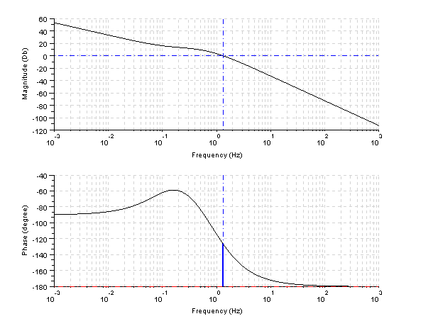
clf;
show_margins(gs);
Results:
 fcg  =
 
    1.1035521  
 mf  =
 
    61.378401
As see, exist a little gain error by the approximation with respect to book

Let's do the program 9.4

Scilab program:
s=%s;
g=10*(s+0.1)/((s+0.5)*s*(s+1));
w=0.5:0.01:1.15;
gs=syslin('c',0.13*g);
gs2=syslin('c',0.188*g);
gr=horner(gs,%i*w);
gr2=horner(gs2,%i*w);
theta=atan(imag(gr),real(gr));
theta2=atan(imag(gr2),real(gr2));
ro=abs(gr);
ro2=abs(gr2);
clf;
k=0:0.01:2*%pi;
nr=cos(k)+%i*sin(k);
theta3=atan(sin(k),cos(k));
ro3=abs(nr);
polarplot([theta3 theta2],[ro3 ro2]);