16 Example 9.2 OGATA 4ed(lag compensator, Bode and Nyquist plot)

Laplace.T	Root-locus	Transient response	Frecuency response

16 Example 9.2 OGATA 4ed(lag compensator, Bode and Nyquist plot)
Let's calculate the lag compensator. Checks and calculations by Scilab.

$\begin{displaymath}G(s)=\frac{1}{s\cdot (s+1)\cdot (0.5s+1)}\end{displaymath}$

We want $K_{v}=5$ ,phase margin $\geq 40$ and gain margin $\geq 10dB$

Solution:
We calculate the constant $K=K_{c}\cdot \beta$ .

$\begin{displaymath}\lim_{s\rightarrow 0}\left( s\cdot G(s) \cdot K_{c} \cdot \be... ...ta \cdot \frac{(T\cdot s+1)}{(T\cdot \beta\cdot s+1)} \right)=5\end{displaymath}$

$\begin{displaymath}K=K_{c} \cdot \beta=5 \end{displaymath}$

$\begin{displaymath}G_{1}(s)=\frac{5}{s\cdot (s+1)\cdot (\frac{s}{2}+1)}\end{displaymath}$
We draw bode plot of $G_{1}(jw)$
Gain table:

$\begin{displaymath}20\cdot log(5)=13.98\end{displaymath}$

w 1 2

$\frac{1}{jw}$ (-20) 0 (-20) (-20)

$\frac{1}{ jw+1}$ (0) 0 (-20) 0 (-20)

$(\frac{jw}{2}+1)$ (0) 0 (0) 0 (-20)

(-20) 13.98 (-40) 1.94 (-60)

$\begin{displaymath}dB\vert G_{1}(j0.1)\vert=20\cdot log(5)-20\cdot log(0.1)=33.98\end{displaymath}$

$\begin{displaymath}dB\vert G_{1}(j1)\vert=20\cdot log(5)-20\cdot log(1)=13.98\end{displaymath}$

$\begin{displaymath}dB\vert G_{1}(j2)\vert=dB\vert G_{1}(j1)\vert-40\cdot log(2)=1.94\end{displaymath}$

$\begin{displaymath}dB\vert G_{1}(j20)\vert=dB\vert G_{1}(j2)\vert-60\cdot log(\frac{20}{2})=- 58\end{displaymath}$

Phase table

w 0.1 0.2 1 2 10 20

$\frac{1}{s}$ -90 (0) -90 (0) -90 (0) -90 (0) -90 (0) -90

$\frac{1}{ s+1}$ 0 (-45) (-45) -45 (-45) (-45) -90 (0) -90

$\frac{1}{\frac{s}{2}+1}$ 0 (0) 0 (-45) (-45) -45 (-45) (-45) -90

-90 (-45) -103 (-90) -166 (-90) -193 (-90) -256 (-45) -270

$\begin{displaymath}\lfloor{G1(j0.2)=-90-45\cdot log(\frac{0.2}{0.1})}=-103.55\end{displaymath}$

$\begin{displaymath}\lfloor{G1(j1)}=-90-45\cdot log(\frac{0.2}{0.1})-90\cdot log(\frac{1}{0.2})=-166.45\end{displaymath}$

$\begin{displaymath}\lfloor{G1(j2)}=-90-45\cdot log(\frac{0.2}{0.1})-90\cdot log(\frac{2}{0.2})=-193.54\end{displaymath}$

$\begin{displaymath}\lfloor{G1(j10)}=-90-45\cdot log(\frac{0.2}{0.1})-90\cdot log(\frac{10}{0.2})=- 256.45\end{displaymath}$

Checks and Bode plot by Scilab
w1=[0.1 1 2 100];
w2=[0.1 0.2 1 2 10 20 100];

gdb1=20*log10(5)
gdb(1)=gdb1-20*log10(0.1)
gdb(2)=gdb1
gdb(3)=gdb1-40*log10(2)
gdb(4)=gdb(3)-60*log10(100/2);

a(1)=-90;
a(2)=-90-45*log10(0.2/0.1);
a(3)=a(2)-90*log10(1/0.2);
a(4)=a(2)-90*log10(2/0.2);
a(5)=a(2)-90*log10(10/0.2);
a(6)=-270
a(7)=-270

s=%s/(%pi*2);
g=1/((s+0.00000000000000001)*(s+1)*(0.5*s+1));
gs=syslin('c',g);
w=logspace(-1,2,100);
gsf=tf2ss(5*gs);
[frq1,rep] =repfreq(gsf,w);
[db,phi]=dbphi(rep);
[gm,fcf]=g_margin(gs)
[pm,fcg]=p_margin(gs)

clf;
subplot(2,1,1);
plot2d(w,db,5,logflag="ln")
plot2d(w1,gdb,2,logflag="ln")
legends(['Exactly','Calculated (approximate)'],[5,2],opt=1);
xgrid;
subplot(2,1,2);
plot2d(w,phi,5,logflag="ln")
plot2d(w2,a,2,logflag="ln")
xgrid;
Results:
-->[gm,fcf]=g_margin(gs)
 fcf  =
 
    1.4142242  
 gm  =
 
    9.5425554  
 
-->[pm,fcg]=p_margin(gs)
 fcg  =
 
    0.7493683  
 pm  =
 
    32.613862
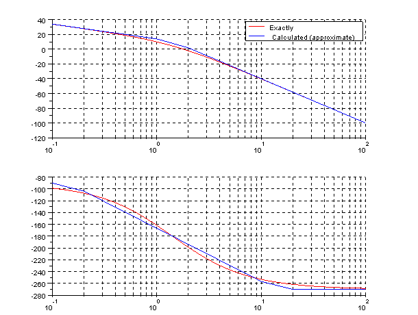
As you see, the phase and gain margins of G(jw) verify the requirements (gain margin is 9.54, with the lag compensator is compensated). Only we need compensate $K_{v}$ . We need a lag compensator.
Let's calculate the frequency at which the phase margin is::

$\begin{displaymath}\phi_{m}=-180º+40º+12º=-128º\end{displaymath}$

$\begin{displaymath}-128=-90-atan(w)-atan(\frac{w}{2})\end{displaymath}$

$\begin{displaymath}-38=-atan(w)-atan(\frac{w}{2});38=atan(w)+atan(\frac{w}{2})\end{displaymath}$

$\begin{displaymath}tg(38)=\frac{w+\frac{w}{2}}{1-w\cdot \frac{w}{2}}=\frac{\frac{3\cdot w}{2}}{\frac{2-w^{2}}{2}}=\frac{3\cdot w}{2-w^{2}}\end{displaymath}$

$\begin{displaymath}2\cdot tg(38)-tg(38)\cdot w^{2}-3\cdot w=0\end{displaymath}$

$\begin{displaymath}w=0.46\end{displaymath}$

This is the new gain crossover frequency

Let's calculate $\frac{1}{T}$ of the compensator. It is a decade below to new gain crossover frequency $\frac{1}{T}=\frac{0.46}{10}=0.046$ so

Let's calculate $\beta$ . First we calculate the gain at the new gain crossover frequency.

$\begin{displaymath}20\cdot log(5)-20\cdot log(0.46)=20.72dB\end{displaymath}$

$\begin{displaymath}20\cdot log(\frac{1}{\beta})=-20.72;log(\frac{1}{\beta})=\frac{-20.72}{20}=-1.04\end{displaymath}$

$\begin{displaymath}\frac{1}{\beta}=0.09;\beta=10.86\end{displaymath}$

So the compensator is:

$\begin{displaymath}\frac{s+\frac{1}{21.74}}{ s+\frac{1}{\beta \cdot 21.74}}=\frac{s+\frac{1}{21.74}}{ s+\frac{1}{236}}\end{displaymath}$

Finally we calculate the $K_{c}$

$\begin{displaymath}K_{c}=\frac{5}{10.86}=0.46\end{displaymath}$

$\begin{displaymath}G_{c}=0.46\cdot \frac{s+\frac{1}{21.74}}{ s+\frac{1}{236}}\end{displaymath}$
Scilab program(Polar plot, margins and Bode plot)
clf;
s=%s;
s1=s/(2*%pi)
g=1/((s1+0.000000000000000001)*(s1+1)*(0.5*s1+1));
gc=0.46*(s1+(1/21.74))/(s1+(1/236));
g1=1/(s*(s+1)*(0.5*s+1));
gc1=0.46*(s1+(1/21.74))/(s1+(1/236));
gt=g*gc;
gt1=g1*gc1;
gs=syslin('c',g);
gts=syslin('c',gt);
gt1s=syslin('c',gt1);
ged(1,1)
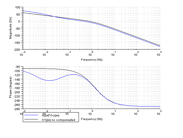
clf;
bode([gs;gts],['G(jw)*Gc(jw)';'G1(jw) no compensated']);
ged(1, 2)
[mg,fcf]=g_margin(gts)
[mp,fcg]=p_margin(gts)
kv=horner(s*gt1s,0)
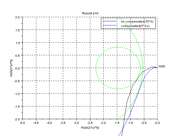
clf;nyquist([gs;gts],['no compensated(10*G)';'compensated(G*Gc)']);
m_circle([1.6;5]);
mtlb_axis([-5 0 -2 2]);
xgrid;
Results:
-->[mg,fcf]=p_margin(gts)
 fcf  =
 
    1.3692079  
 mg  =
 
    15.724625  
 
-->[mp,fcg]=p_margin(gts)
 fcg  =
 
    0.4179369  
 mp  =
 
    49.815168 
  kv  =
 
    4.9935603
The compensated system verify the conditions of Kv,gain and phase margins.
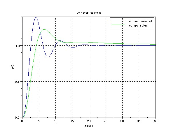
Scilab program to draw the unit-step response
clf;
s=%s;
g=1/(s*(s+1)*(0.5*s+1));
gc=0.46*(s+(1/21.74))/(s+(1/236));
gt=g*gc;
gc=g /. 1;
gtc=gt /. 1;
gs=syslin('c',gc);
gts=syslin('c',gtc);
t=0:0.02:40;
y=csim('step',t,gs);
yt=csim('step',t,gts);
plot(t,y);
plot(t,yt,'g')
xgrid;
legend(['no compensated';'compensated'])
xtitle('Unit-step response','t(seg)','y(t)')
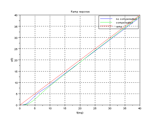
Scilab program to draw ramp response
clf;
s=%s;
g=1/(s*(s+1)*(0.5*s+1));
gc=0.46*(s+(1/21.74))/(s+(1/236));
gt=g*gc;
gc=g /. 1;
gtc=gt /. 1;
gs=syslin('c',gc);
gts=syslin('c',gtc);
t=0:0.02:40;
y=csim(t,t,gs);
yt=csim(t,t,gts);
plot(t,y);
plot(t,yt,'g');
plot(t,t,'r');
xgrid;
legend(['no compensated';'compensated';'ramp'])
xtitle('Ramp response','t(seg)','y(t)')