clf;
s=%s/(%pi*2);
g=4/(s*(s+2));
gc=41.7*(s+4.41)/(s+18.4);
gt=g*gc;
gs=syslin('c',10*g);
gts=syslin('c',gt);
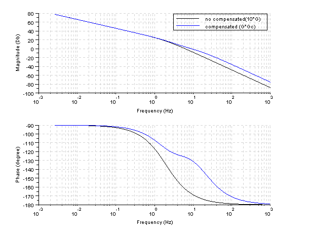
clf;
bode([gs;gts]);
legend(['no compensated(10*G)';'compensated (G*Gc)'])
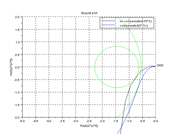
Scilab program (polar plot)
clf;
s=%s/(2*%pi);
g=4/(s*(s+2));
gc=41.7*(s+4.41)/(s+18.4);
gt=g*gc;
gs=syslin('c',10*g);
gts=syslin('c',gt);
clf;
nyquist([gs;gts],['no compensated(10*G)';'compensated (G*Gc)']);
m_circle([1.9;10]);
mtlb_axis([-5 0 -2 2]);
xgrid;
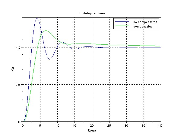
Scilab program (unit-step response) by Scilab
clf;
s=%s;
g=4/(s*(s+2));
gc=41.7*(s+4.41)/(s+18.4);
gt=g*gc;
gc=g /. 1;
gtc=gt /. 1;
gs=syslin('c',gc);
gts=syslin('c',gtc);
t=0:0.02:6;
y=csim('step',t,gs);
yt=csim('step',t,gts);
plot(t,y);
plot(t,yt,'g')
xgrid;
legend(['no compensated';'compensated'])
xtitle('Unit-Step response','t(seg)','y(t)')
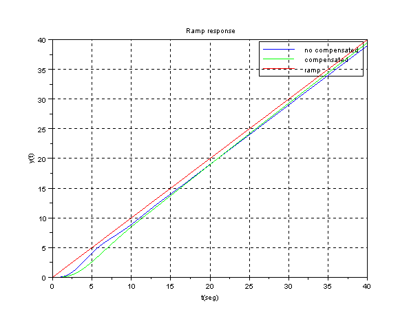
Scilab program (Ramp response)
clf;
s=%s;
g=4/(s*(s+2));
gc=41.7*(s+4.41)/(s+18.4);
gt=g*gc;
gc=g /. 1;
gtc=gt /. 1;
gs=syslin('c',gc);
gts=syslin('c',gtc);
t=0:0.02:6;
y=csim(t,t,gs);
yt=csim(t,t,gts);
plot(t,y);
plot(t,yt,'g');
plot(t,t,'r');
xgrid;
legend(['no compensated';'compensated';'ramp'])
xtitle('Ramp response','t(seg)','y(t)')