XML
Laplace.T Root-locus Transient response Frecuency response


18 Problem A9.5 OGATA 4ed(Lead compensator, Nichols chart)


    Let's insert a compensator for the open-loop system is tangent to circle M=3dB in w=3rad/seg. The open-loop system is the following:

    \begin{displaymath}G(s)=\frac{1}{s^2}\end{displaymath}


    G (s) is the phase constant at -180 and the gain varies depending on the frequency. 
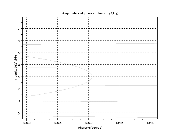
We will draw Nichols for M = 3 dB


    Scilab program
    
    clf;
    chart(3);
    mtlb_axis([-230 -130 -5 15])
    xgrid;
    
    Image ProblemaA9_5

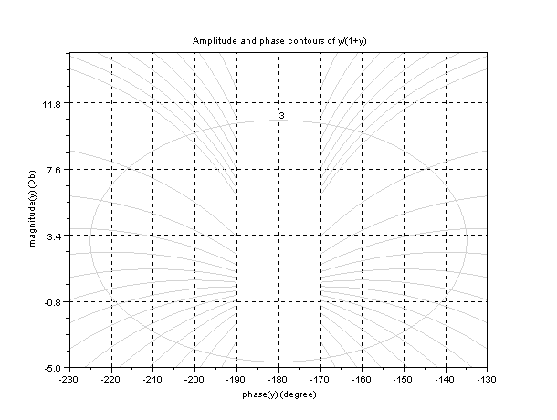
    As we can see that the system is tangent, has to move to a phase of -135. $180-135=45$ degrees. Ie we have to introduce a lead compensator compensates us 45 degrees.

    \begin{displaymath}sen 45=\frac{1-\alpha}{1+\alpha}\end{displaymath}


    \begin{displaymath}\alpha=\frac{1-sen(45)}{1+sen(45)}=0.17\end{displaymath}


    \begin{displaymath}Gc(s)=K_{c} \cdot \frac{s+\frac{1}{T}}{s+\frac{1}{\alpha \cdot T}}=K_{c} \cdot \frac{s+\frac{1}{T}}{s+\frac{1}{0.17 \cdot T}}\end{displaymath}


    We know that the tangent frequency at 45 degrees is 3rad/seg as the frequency where the compensation is maximum (where the open loop system has to be tangent).

    \begin{displaymath}w=\frac{1}{\sqrt{\alpha}\cdot T};\frac{1}{T}=w\cdot \sqrt{\alpha}=3\cdot \sqrt{0.17}=1.24\end{displaymath}


    \begin{displaymath}Gc(s)=K_{c} \cdot \frac{s+1.24}{s+\frac{1.24}{0.17}}=K_{c} \cdot \frac{s+1.24}{s+7.24}\end{displaymath}


    Now we have to calculate $ K_ (c) $ knowing that the gain has to be 3dB. If we see an expansion of the Nichols chart above that the tangent point in the gain will be 3dB.
    Image ProblemaA9_5b

    \begin{displaymath}20 \cdot log10\vert G(j3)\cdot G_{c}(3j)\vert=20 \cdot log10\...
... \frac{3j+1.24}{3j+7.24}\vert=20\cdot log10(K_{c}\cdot 0.046)=3\end{displaymath}


    \begin{displaymath}K_{c}\cdot 0.046=10^{\frac{3}{20}}\end{displaymath}


    \begin{displaymath}K_{c}=30.7\end{displaymath}


    \begin{displaymath}G_{c}=22.79 \cdot \frac{s+0.8}{s+4.69}\end{displaymath}


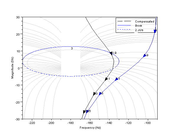
    We will draw plots Nichols of results with Scilab
    s=%s/(2*%pi);
    g=1/s^2;
    gc=30.7*(s+1.24)/(s+7.24);
    gc2=5.19*(0.816*s)/(0.136*s+1);
    gt=g*gc;
    gt2=g*gc2;
    gts=syslin('c',gt);
    gts2=syslin('c',gt2);
    clf;
    chart(3);
    black([gts;gts2],['Compensated';'Book']);
    mtlb_axis([-230 -90 -30 30])
    
    Image ProblemaA9_5c