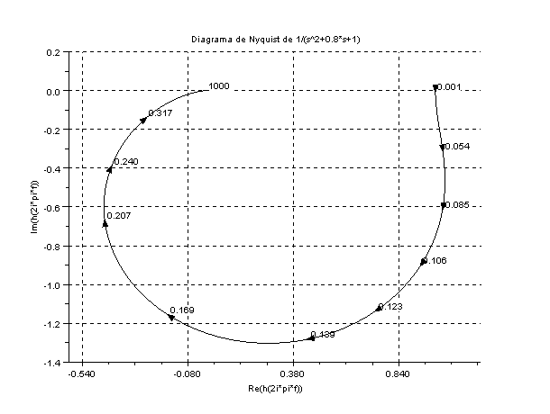
3 Example 8-10 OGATA 4ed(Nyquist plot) Let's plot Nyquist plot by Scilab. Scilab program clf; s=%s/(2*%pi); g=1/(s^2+0.8*s+1); gs=syslin('c',g); nyquist(gs); xgrid; xtitle('Nyquist plot of 1/(s^2+0.8*s+1)') As we see we only plot the part that goes to . Let's do it from to Scilab program clf; s=%s/(%2*pi); s1=-s; g=1/(s^2+0.8*s+1); g1=1/(s1^2+0.8*s1+1); gs=syslin('c',g); gs1=syslin('c',g1); nyquist(gs); nyquist(gs1); mtlb_axis([-2 2 -2 2]) xtitle('Nyquist plot of 1/(s^2+0.8*s+1)')
clf;

s=%s/(2*%pi);

g=1/(s^2+0.8*s+1);

gs=syslin('c',g);

nyquist(gs);

xgrid;

xtitle('Nyquist plot of 1/(s^2+0.8*s+1)')
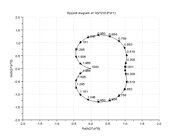
Let's do it from to
clf;

s=%s/(%2*pi);

s1=-s;

g=1/(s^2+0.8*s+1);

g1=1/(s1^2+0.8*s1+1);

gs=syslin('c',g);

gs1=syslin('c',g1);

nyquist(gs);

nyquist(gs1);

mtlb_axis([-2 2 -2 2])

xtitle('Nyquist plot of 1/(s^2+0.8*s+1)')