2 Example 8-6 OGATA 4ed (Bode plot)

Laplace.T	Root-locus	Transient response	Frecuency response

2 Example 8-6 OGATA 4ed(Bode plot)

Let's plot Bode plot by Scilab.

$\begin{displaymath}G(s)=\frac{9\cdot (s^{2}+0.2\cdot s+1)}{s\cdot(s^{2}+1.2\cdot s+9)}\end{displaymath}$

Scilab program

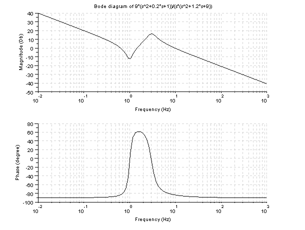
s=%s;
s1=s/(2*%pi);
g=9*(s1^2+0.2*s1+1)/(s1*(s1^2+1.2*s1+9));
gs=syslin('c',g);
clf;
w=logspace(-2,3,100);
bode(gs,w);
xtitle('Bode plot of 9*(s^2+0.2*s+1))/(s*(s^2+1.2*s+9))');

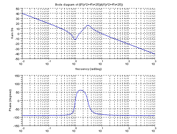
Let's do it but according as program 8.4

Scilab program

s=%s/(2*%pi);
g=(9*(s1^2+0.2*s1+1))/(s1*(s1^2+1.2*s1+9));
gs=syslin('c',g);
w=logspace(-2,3,100);
gsf=tf2ss(gs);
[frq1,rep] =repfreq(gsf,w);
[db,phi]=dbphi(rep);
clf;
subplot(2,1,1);
plot2d(w,db,style=0,logflag="ln")
plot2d(w,db,style=2,logflag="ln")
xgrid;
mtlb_axis([0.01 1000 -50 50]);
xtitle('Bode plot of (9*(s^2+4*s+25))/(s*(s^2+4*s+25))','frequency (rad/seg)',
'Gain Db')
subplot(2,1,2);
plot2d(w,phi,style=0,logflag="ln")
plot2d(w,phi,style=2,logflag="ln")
xtitle('','frequency (rad/seg)','Phase (degrees)');
mtlb_axis([0.01 1000 -150 150]);
xgrid;